

Conceptual Framework
Variations in river flow tend to decrease with increasing area of consideration, partly due to a decrease in temporal correlation of rainfall events across space. Patchiness of rainfall can contribute to an increase of yield stability over space. Existing rainfall simulators tend to focus on station-level time series, not on space/time autocorrelation.
The SpatRain model described here was constructed to generate time series of rainfall that are fully compatible with existing station-level records of daily rainfall, but yet can represent substantially different degrees of spatial autocorrelation. Calculations start from the assumed spatial characteristics of a single rainstorm pathway, with a trajectory for the core area of the highest intensity and a decrease of rainfall intensity with increasing distance from this core. The model can derive daily amounts of rainfall for a grid of observation points by considering the possibility of multiple storm events per day, but not exceeding the long-term maximum of observed station-level rainfall. Options exist for including elevational effects on rainfall amount. SpatRain is implemented as an Excel workbook with macros that analyze semivariance as a function of increasing distance between observation points, as a way to characterize the resulting rainfall patterns accumulated over specified lengths of time (day, week, month, year).
• Assumed
storm properties
• Synchronizing spatial pattern with temporal pattern
• Considering multiple storm events
• Storm events probability
• Considering elevational effect
• Patchiness indicator
Three parameters are used for describing rainfall in the core area: the length of the core trajectory, the width of the core area and the rainfall depth in the core area. Two further parameters describe the relative decrease of rainfall depth with increasing distance from the core. The combination of these can produce the full scale of ‘homogenous’ to ‘heterogeneous’ types of rain. These parameters can be related to frictional forces forming thunderstorms or convective bands causing frontal circulation. Thus, intensity from the core is calculated as follows:
![]() .....................................................................................(1)
.....................................................................................(1)
where:
d is distance of a cell from the storm core (grid unit);
Id is rain intensity of a cell at distance d from the core (mm.d-1);
I0 is rain intensity at the core (mm.d-1);
f? is spreading factor; and
f? is agglomerating factor.
Synchronizing spatial pattern with temporal pattern
A single storm event will ‘wet’ (above the measurement threshold of 0.5 mm day-1 used in most empirical data sets) a number of cells, some at the core intensity and some at a lower intensity. Given a set of parameters for the storm trajectory, we can derive the frequency distribution of rain depth in wetted cells, relative to the core rain intensity (p), in n classes. Once this is known, the frequency distribution of core intensities (F) can be derived from the observed station level rain intensities (f). Frequency distributions of f, p and F should have the same class number and interval order. We use the following order to define the class boundary: [max..max*q1],[ max*q1.. max*q2], [max*q2.. max*q3],…,[ max*qn.. min], where max is the maximum data, min is the minimum data and n is class intervals number. The value of q is ranging from 0 to 1 and calculated as follows:
![]() .....................................................................................(2)
.....................................................................................(2)
![]() ..............................................(3)
..............................................(3)
We first need to recognize the combinations of classes pj and Fk that are compatible with class fi:
For the highest rainfall class only one combination, involving the highest class of both p and F will yield the desired result, but for the other classes there can be several combinations of p and F that yield the same result (the tail end of a big rainfall event, a medium fraction of a medium storm or the core area of a small storm). We can approach it working our way from the top down, but a simpler derivation starts from the observation that for all distributions f, p and F the sum equals 1. By assuming that the resultant (f) comes from the multiplication between p and F, we then get this basic equation:
![]() ..................................................................................................................(4)
..................................................................................................................(4)
So that F
of frequency class n can be defined as:
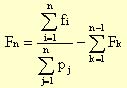 .................................................................................................................(5)
From the
equation, we can derive a criterion for the shape of the p distribution
(that depends on assumed storm properties) that is compatible with the
targeted f distribution. If at any point ![]() is
less than
is
less than ![]() Fn would violate the
assumption of non-negative subsequent F terms. So, a cross-over of p and
f indicates incompatibility of the storm-level assumptions ? that generate
the p curve ? with the station-level rainfall records ? that generate
the f curve. Figure 3 illustrates the compatibility of intensity distribution
from two contrasting spatial patterns of 30-grid maps with temporal distribution
from 30-day station record. Pattern B of exactly similar distribution
to the station record rainfall produces compatible F as shown in figure
3D, whereas pattern C is incompatible with the station record distribution
as indicated by negative values of F in figure 3E. This means, it is impossible
to arrange rainfall maps of pattern C using the existing temporal distribution.
Fn would violate the
assumption of non-negative subsequent F terms. So, a cross-over of p and
f indicates incompatibility of the storm-level assumptions ? that generate
the p curve ? with the station-level rainfall records ? that generate
the f curve. Figure 3 illustrates the compatibility of intensity distribution
from two contrasting spatial patterns of 30-grid maps with temporal distribution
from 30-day station record. Pattern B of exactly similar distribution
to the station record rainfall produces compatible F as shown in figure
3D, whereas pattern C is incompatible with the station record distribution
as indicated by negative values of F in figure 3E. This means, it is impossible
to arrange rainfall maps of pattern C using the existing temporal distribution.
Considering multiple storm events
Equation 1 may produce a narrow-spread area of single storm events, on which its wet cells ratio relative to total area (c1) does not match the wet days fraction of that specific month (d). Hence, we need to allow for multiple storm events, depending on the area fraction wetted by a single event and the time fraction of rainy days at the measurement station level. For spatially independent multiple events on a single day we can derive that probability of dry days on a given month, P|?|, should meet the probability of dry cells during single event, P|?|, to the power of events number (N):
![]() .....................................................................................................(6)
.....................................................................................................(6)
Where P|![]() |=1-d and P|
|=1-d and P|![]() |=1-c1.
Thus, the number of events is:
|=1-c1.
Thus, the number of events is:
![]() ...........................................................................................................................(7)
...........................................................................................................................(7)
Patchy rains have less wet fraction than homogeneous rains in space. In order to conserve each cell to having uniform chance of being hit by storms in time, patchy rains should have higher probability to occur than homogeneous rains. Consequently, the probability of storm with N number of events (P(EN)) is defined from wet days fraction (d) by taking wet cells fraction of N storm events (cN) into account:
![]() ...........................................................................................................................(8)
...........................................................................................................................(8)
Considering elevational effect
Rainfalls
at particular degree of patchiness generated by the above procedures should
be corrected if applied on an area with elevational effects. The elevation
modifier of rainfall at elevation z (Xz) is assumed as rainfall average
at that elevation (![]() z) relative
to reference station (
z) relative
to reference station (![]() ):
):
![]() ..................................................................................................................................(9)
..................................................................................................................................(9)
In fact we are modifying the amount of rain that any storm brings to any cell, not the preferred pathway of storm trajectories. Though similar multipliers we can introduce ‘rain shadow’ effects that depend on a preferential direction of storms and gradients in elevation.
Semivariogram is used as quantitative spatial pattern indicator of simulated rainfall. It is expected that homogenous rainfalls will have longer range than patchy rainfalls.