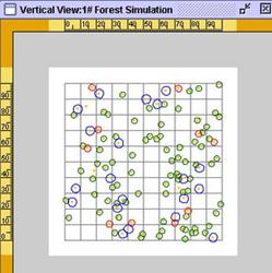
4. Simulation Results

You can explore the simulation output by either inspecting the tree plotting in Two Dimension (2D) and Three Dimension (3D) graphic or plotting the tree data on statistical chart.

4.1. Vertical Projection 2D of Tree Plot

You can access the shortcut to view vertical projection from simulation menu (see section Simulation Menu).

Figure 69: Vertical Projection Option

Figure 70: Vertical View Window

4.1.1. Tree Paint Options

You can set the tree painting on the 2D plot by right click the plot, select “paint”.

Figure 71 2D Tree Paint Options Menu

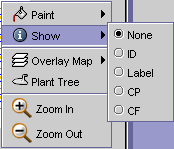
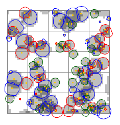
Default option is paint with Outline mode. You can reset either with opaque, transparent, or shading mode.

4.1.2. Tree’s Info

You can view the basic info of the plotted trees by selecting the “Show” menu. You can show either the ID, Species Label, CP index or CF index. see Figure 75.

Figure 72: Show Tree’s Info menu

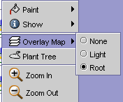
4.1.3. Overlay Map

The plot can be overlay with either “Light Map” Layer or “Root Influential Zone Map” Layer. To set the overlay map, select “Overlay Map” on simulation menu,

Figure 73.

Figure 73 Overlay Map Option Menu Figure 74 Light Map (left) and Root Map (Right) Overlay

4.1.4. Cut the Trees

On Vertical Projection Plot you can cut (remove) the trees. Select the trees, Right click, and Select “Remove”. Note that those removed trees are also removed from the simulation and counted as mortality data.

Figure 75: Remove Tree in Vertical View

4.1.5. Tree’s Object Inspector

This menu will show the technical properties of Tree Object.

Figure 76: Object Inspector Option Figure 77: Object Inspector

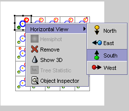
4.2. Horizontal Projection 2D of Tree Plot

To view the trees on horizontal projection, select the tree from Vertical Projection Plot, Right click and select “Horizontal View”. You can view the projection either from North, South, West or East side.

Figure 78: Horizontal Projection View

Figure 79 Horizontal View Menu

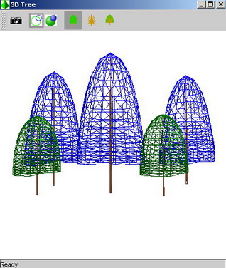
4.3. View 3D Visualization

You can explore the tree in 3D Graphics. Make sure that you have minimum requirement for viewing the 3D graphics (see section Minimum Requirement). You can access the 3D Visualization shortcut from Simulation Menu

Figure 80: 3D View in Simulation Menu

Figure 81: Virtual Forest Setting.

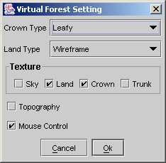
After you select the “3D View” menu, the Virtual Forest Setting dialog will appear ( Figure 81).

The 3D visualization setting options are:

• Crown type
  You can set the Tree Crown rendering type either using Wireframe, Solid or Leafy modes.
• Land Type
  You can set also the Land rendering either using Wireframe or Solid modes.
• Texture
  Texture rendering can be applied for each 3D components: Sky, Land, Crown and Trunk
• Topography
  Check if you want to enable the topography rendering on 3D Visualization (make sure that you have applied the topography data)
• Mouse Control
  Check if you want to enable moving the 3D Objects using the mouse.

Figure 82: Wireframe Crown and Land in Virtual Forest


Figure 83: Leafy and Textured Tree Crown 3D visualization

Figure 84:Virtual Control Window

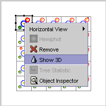
4.4. View 3D Animation

Select a tree or a group of trees on Vertical Projection View window, Right click, and select show 3D (Figure 85). Make sure you have enabled the “Record Tree Profile History” option on Simulation Plot Setting (Section 3.2)

Figure 85: 3D Option Menu from Vertical View Window

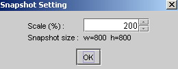
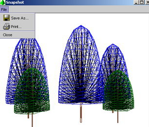
4.5. 3D Visualization Window Menus

The 3D window shortcut menus are:

4.5.1. Snaphot

Click here to capture the image from 3D Visualization. Set the scaling factor then click Ok. The snapshot window will show up. After, you can either save the image or print it .

Figure 86: Snapshot Setting Box

Figure 87: Snapshot Window

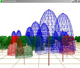
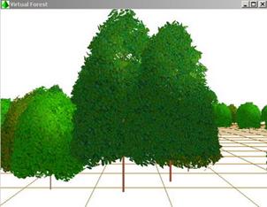
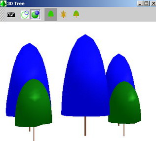
4.5.2. Rendering Mode

You can set the rendering mode of the 3D Visualization either using wireframe or solid mode

Figure 88: Tree in Transparent Mode

Figure 89:Tree in Solid Mode

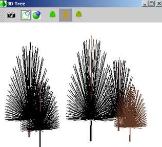
4.5.3. Show 3D Component Part

You set the 3D Visualization to show the part of object. You can set either just showing the crown layer ( ), the branches ( ) or both crown layer and branches ( ).

Figure 90: Tree Branches View

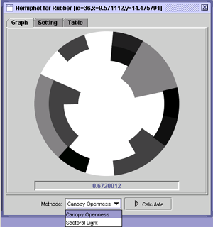
4.6. Hemispherical Photograph

You can view hemispherical photograph model of canopy gap from a tree point of view. Select a tree on Vertical Projection Plot, Right click, and select “Hemiphot”. The hemiphot window will show up (Figure 92).

Figure 91: Hemiphot Menu in Vertical View Window

Figure 92 Hemiphot Window

There are two type of hemiphot map:

• Canopy openness
  This represents the canopy openness computed at crown base assuming target tree crown is completely transparent
• Sectoral Light .
  Sector light is a smoothed map of canopy openness used to compute anisotropic gradient affecting crown deformation

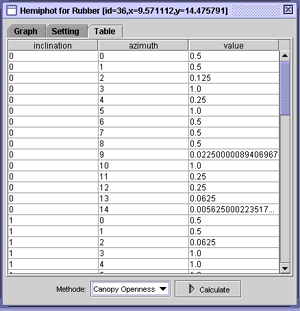
You can try to change the light insolation setting for current hemiphot position by opening the “Setting” tab. click Calculate button to refresh the hemiphot after you change the setting.

You can view the detail value of each hemiphot sector by opening the “Table” tab.

Figure 93: Hemiphot Table

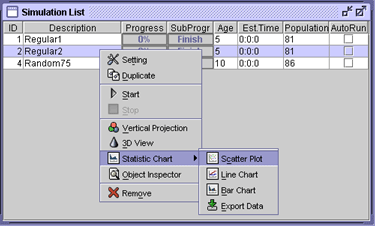
4.7. Statistical Data

Statistical data output can be accessed either for overall simulation list, for selected simulation or for each individual tree. To view overall simulation list statistical data, open the “Statistical Chart” menu on the Main Window menu bar and select the type of the chart.

Figure 94: Statistic Chart Menu for Overall Simulation List

To view the statistical data for each simulation items, select (Highlight) the simulation item on the simulation list window, right click and select “Statistic Chart”.

Figure 95: Data Option in Simulation Options

To view statistical data of individual tree, select a tree on the vertical projection plot, Right click, then select “Tree Statistic” (Figure 104).

Figure 96: Tree Stat Option

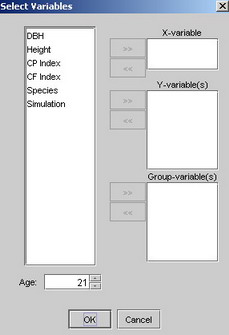
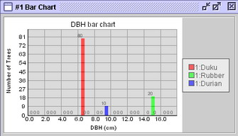
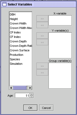
4.7.1. Bar chart

Select the variable on the left panel and move it to the x axis panel on the right. The available x axis variables are DBH (Diameter at Breast Height), Height, CP Index, CF Index.

“Species” and “Simulation” are the grouping variables.

You can view the simulation data of any age by setting the Age field.

Figure 97: Bar Chart Variables

Figure 98: Bar Chart

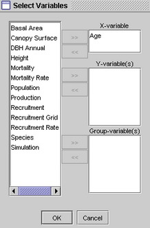
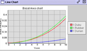
4.7.2. Line chart

The available variables for Y axis in line charts are: Basal Area (Cross sectional area of tree), Crown surface, DBH annual, Height, Mortality (number of deaths over a specific time period), Mortality rate (Mortality relative to the population size), Population, Production (fruit, timber, latex, or resin), Recruitment (the count of new members into a population), Recruitment Grid (Number of available grid cells suitable for recruitment of each species), Recruitment Rate.

Species and Simulation are the group variable

The X axis variable is Age.

Figure 99: Line Chart Variables

Figure 100: Basal Area in Line Chart

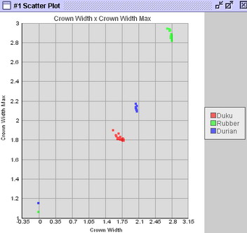
4.7.3. Scatter plot

The available variable for X and Y axis are: DBH, Height, Crown Width (2 * Geometric means of crown radius), Crown Width Max (2 * Max Crown Radius), CP Index, CF Index, Crown Depth, Crown Depth Ratio (Crown Depth/height), Production.

Species and Simulation are the group variable.

Figure 101: Scatter Plot Variables

Figure 102: Scatter Plot