3. User's Manual

3.1. Create New Simulation

There are several ways to create a simulation. These are:

1. On the menu bar click Add New menu bar.
2. In the File Menu, select New Simulation menu.

After you gone through one of those steps, the Create New Simulation Wizard will show. Follow these steps:

• On Source Simulation dialog, you will be asked whether you want to load an existing simulation or create a new simulation.
  If you choose to load an existing simulation, the Browse button will be active, and you can browse your computer to search for the saved file.
  
  
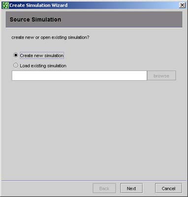
  Figure 22: Source Simulation Dialog
  
• Click Next button, and Simulation Description dialog will show.
  In this wizard dialog, the simulation’s description will show. You may change simulation’s Name and Area Size. The area size default is 100x100 m.
  
  
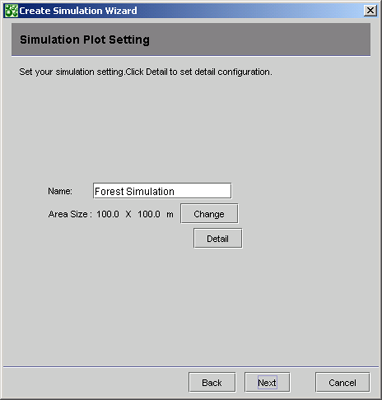
  Figure 23:Simulation Description Dialog
  
  Clicking on “Detail” will show up the detail setting for the plot, Aboveground and Belowground Setting. The explanation about those parameters is to be found in section Simulation Plot Setting.
  
  
  Figure 24 Aboveground Setting
  
  
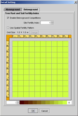
  Figure 25 Belowground Setting
  
• After the plot setting, Clicking Next button will bring you to Tree Species Setting.
  Add the species by clicking button. The species description item will be added to the list. Then, double click on the species item that you have added and the detail setting for the species will show up. Detail explanation about species parameter is covered under section Species Parameter Setting section
  
  Click to remove selected species and click on to remove ALL species in the list. If you have previously saved species descriptions then click to load the species description file. And click on "Save" button to save the current species list into a file.
  
  
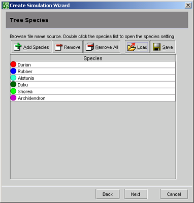
  Figure 26: Tree Species Setting Dialog
  
  
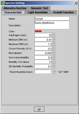
  Figure 27 Detail Species Setting
  
• Click Next button to go to Initial Planting Area dialog.
  There are three ways to plant the trees into the plot: plant randomly, manually, or orderly. Detail explanation about this Initial Plantation is given in section 3.5. Initial Stand.
  
  
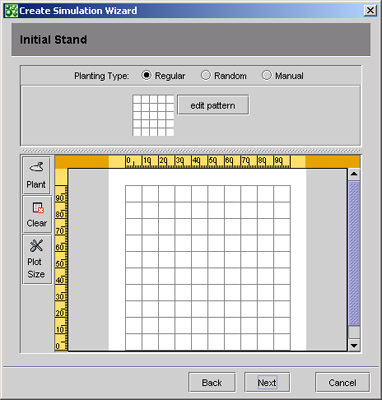
  Figure 28: Initial Stand Dialog
  
• Click Next button, and the Summary dialog will show.
  The last option is to choose weather you want to run the simulation later or run it immediately.
  The auto run option is for batch mode run.
  
  
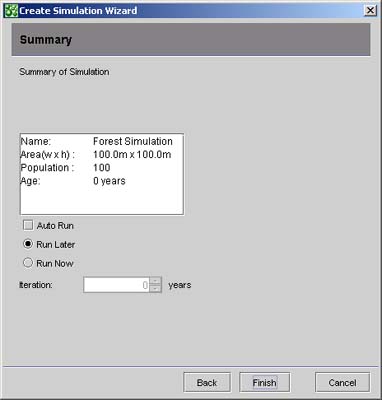
  Figure 29: Summary Dialog
  
  Click Finish button. The simulation description item will be added to the Simulation List window.
  
  
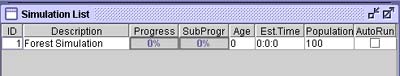
  Figure 30: Simulation List Window

If you choose the “Run Later” option before the simulation plot will be stopped at its initial stage. You can run this simulation by double clicking the simulation item on the list, and The Simulation Control window will show up (Figure 31). Fill the Iteration Setting field with the length of simulation you wish to run in year, then click start button .

Figure 31: Simulation Control Window

You can reset the default setting for the plot and the species by clicking the Setting icon. You access this shortcut by clicking on the “Simulation” menu on the main window or right clicking the simulation description item on the simulation list.

Figure 32: Simulation Menu

Next section will describe in detail the settings for the Simulation Plot and Tree Species.

3.2. Simulation Plot Setting

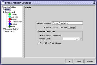
Figure 33: Forest Simulation Panel

In Forest Simulation panel (see Figure 33), you must specify the parameter values to be used, which are:

• Simulation’s Name
  Fill the label for current simulation setting
• Area Size
  The default value for plot area is 100.0 x 100.0 m. Click Change button to change the area size, and the Input New Area Size dialog will show. Type the size of the new area and click OK.
  
  
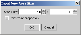
  Figure 34: Area Size
  
• Random Generator
  Type the random seed for the Random Generator. It can be any number.
• Record Tree Profile History
  Check if you want to record the tree profile history and show it in 3D visulization

3.2.1. Aboveground Setting

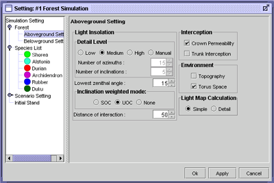
Figure 35:Light Setting Panel

The parameters are:

• Light Insolation
  Light Insolation settings control the level of detail used for exploring the sky vault, i.e. the number of light beams and their weighting. The number of inclinations and azimuths defines the number of beams.
  Azimuth is the horizontal component of a direction (compass direction), measured around the horizon from the North point, toward the East, i.e. clockwise. It is usually measured in degrees.
  Inclination is the angular distance of the orbital plane from the plane of reference (usually planet's equator or the ecliptic), stated in degrees.
  
  
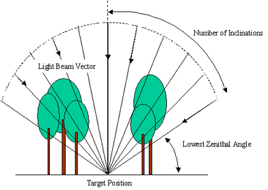
  Figure 36: Horizon Projection of Beams Vector
  
  
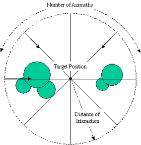
  Figure 37: Vertical Projection of Beams Vector
  
  The parameters for insolation are:
  • q Detail Level
    There are four options of detail level:
    1. Low
       If you choose low, the system will set 5 as number azimuths value, and 3 as number of inclinations..
    2. Medium
       If you choose medium, the system will set 15 as number azimuths value, and 5 as number of inclinations.
    3. High
       If you choose high, the system will set 30 as number azimuths value, and 10 as number of inclinations.
    4. Manual (Inactivated)
       If you choose manual, you can freely set the number of azimuths and number of inclinations.
  • Lowest Zenithal Angle
    Lowest Zenithal Angle defines the lowest angle considered for light calculation.
  • Inclination weighted model
    There are three models you can choose from:
    1. SOC (Standard Overcast Sky)
       This model weights each direction according to surface of sky vault fraction moreover assuming a decrease in light intensity from zenith to horizon, using the formula:
       
    2. UOC (Uniform Overcast Sky)
       This model weights each direction according to the relative surface of the sky vault explored by each beam.
    3. None
       This option gives equal weight to each direction sampled.
  • Distance of Interaction
    The interaction area is limited by the Distance of Interaction setting. The trees outside the radius of interaction distance and are not included for current target calculation.
• Interception
  The parameters for interception are:
  • Crown Permeability
    If Crown Permeability checkbox is selected, the crown is considered as partially transparent (transparency is also referred to as crown porosity in the following). If Crown Permeability is not selected, it is assumed to be totally opaque.
  • Trunk.
    If Trunk Interception checkbox is selected, the trunk is considered to intercept the light. If Trunk Interception is not selected, it’s neglected.
• Environment
  • Topography
    If topography is selected, the plot will using the topography data (if it exists), else the plot is assumed to be flat.
  • Torus Space
    In geometry, a torus (pl. tori) is a doughnut-shaped surface of revolution generated by revolving a circle about an axis coplanar with the circle. The sphere is a special case of the torus obtained when the axis of rotation is a diameter of the circle. If the axis of rotation does not intersect the circle, the torus has a hole in the middle and resembles a ring doughnut, a hula hoop or an inflated tire. The other case, when the axis of rotation is a chord of the circle, produces a sort of squashed sphere resembling a round cushion. Torus was the Latin word for a cushion of this shape.
    If selected then the plot is assumed to be toric, in such case the plot has no borders as the trees from one side of the plot act as neighbors for the trees on the opposite side. If not selected then the plot is limited by the border. (Note that the area outside the border is considered as an open area).
• Light Map Calculation
  There are two options on Light Map Calculation:
  • Simple
    Select Simple if you want to use simple Light Map Calculation
  • Detail
    Select Detail if you want to use detail Light Map Calculation

Light calculation for each grid cell in this module uses Simple Vertical Light Calculation (cf SLIM part below). The plot is divided into a grid of cells (default size 5 by 5 m). For each cell at each time step a coarse index of light availability is computed based on overhead light of target cell and 8 immediate neighbors (a single vertical direction originating from center of cell is explored for each cell).
The average of canopy openness on each grid cell is used in the recruitment process to assess suitability of light regime.

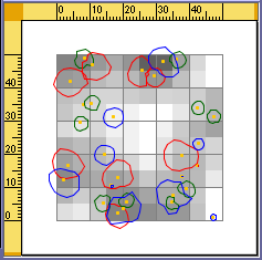
Figure 38: Light Map for Recruitment Test Shown in SExI GUI

3.2.2. Belowground Setting

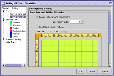
Figure 39: Belowground Setting Panel

Check the Enable Belowground competitions option to simulate below ground competition between neighboring trees. The parameters for root influential zone are explained in section 3.3 Species Parameters Setting.

Soil fertility is set manually for each cell of a grid covering the plot or read from a text file. Missing data are interpolated using bilinear 3 dimensional interpolations (Press, Teukolsky et al. 1992). Fertility values vary between 0 and 1; a fertility of one meaning there is no soil fertility related limitation.

The fertility experienced by a tree will be computed as the average of cells fertility value of cells within the tree root influential zone.

3.3. Species Parameters Settings

3.3.1. Set Species List

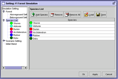
Figure 40 Species Description List

Add species by clicking button. The species description item will be added to the list. Next, double click on the species item that you have added and the detail setting for the species will show up. Detailed explanation about the species parameters is given in Species Parameter Setting section.

Click to remove selected species and Clicking on will remove all species on the list. If you have previously saved species descriptions then click to load the file. And click on “Save” button to save the current species list into a file.

Select the species label on the left tree menu, the right panel will show the detailed species settings for the selected species.

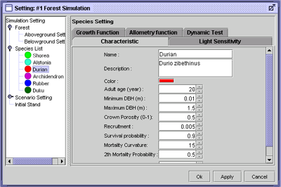
Figure 41: Species Characteristic Setting

3.3.2. Species characteristic

The first tab is species characteristic setting. Except Species Name and Species Description, the parameters are:

• Color.
  The color is used for visualization purposes; it’s not the real color of the tree species. This color is useful to differentiate between species. Click the color to change color.
• Adult age (year)
  Type the age of the tree species when it reaches sexual maturity (determines start of recruitment for non pioneer species, see below)
• Minimum DBH (Diameter at Breast Height)
  Enter the initial diameter for newly recruited trees (default is 1 cm dbh)
• Maximum DBH
  Enter the maximum diameter of the tree species
• Recruitment
  This recruitment rate is the proportion of suitable "gaps” that are filled by a particular species at each time step. It does not depend on number of adult trees of the same species. However it is conditional (for non pioneer species) to the presence of at least one mature adult tree in the stand. Suitability for recruitment is based on minimum and maximum light levels setting. Location of newly recruited seedling/sapling is randomly chosen within the range of suitable locations.
  The minimum and maximum light levels setting for recruitment are defined on "Light Sensitivity" part and Light availability map is calculated using two optional method, accessible under "Forest" > "Light Setting" section.
  This method of recruitment refers to natural regeneration ("Natural Recruitment" scenario) and can be overridden in the management scenario (see below).
• Min Survival Probability
  Min Survival probability (sp) is the survival probability value of a completely suppressed plant (no growth)
  In addition, a systematic mortality is assumed once tree crown size has reached 5% of normal crown size
• Mortality Curvature
  Mortality Curvature modulates the shape of survival probability curve as growth rate is reduced (higher m values imply higher mortality rates at identical growth rate). Default value is 15. See documentation for more details.
• 2nd Mortality Probability
  2nd Mortality Probability is the probability that a tree dies from a neighboring tree fall (0 - 1) if it lies in the sector affected by tree fall. Default value is 50% (see documentation for further computational details).
• Root Influential Zone Modifier
  Species specific factor of root influential zone from default 20*DBH meters

3.3.3. Light Sensitivity

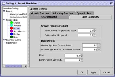
Figure 42: Light Sensitivity Setting

Here are the parameters that define the light stress factor of the tree growth. The curve below shows the light stress factor derived from the parameters:

• Growth response to light:
• Minimum Level for Growth to Occur
  Input the minimum level for a tree so that the tree can grow.
• Optimum Level for Growth
  Input the optimum level for a tree to grow.
  
  
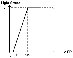
  Figure 43: Light Stress Graphic
  min = Minimum level for growth to occur
  opt = Optimum level for growth
  
• Recruitment
  Once a recruitment decision is made for a tree of a particular species it is randomly “planted” within the area defined as suitable i.e. which light level is between minilum_for_recruitment and maxilum_for_recruitment
• Minimum Light Level for Recruitment
• Maximum Light Level for Requirement to Occur

3.3.4. Growth Function

DBH as the function of time (t) uses a Chapman Richards function:

Approximating DBH annual increment with the first derivative of DBH with respect to time (t) one can express dbh increment as a function of current dbh as follows:

(See SExI-FS Documentation for detail)

The parameter of c and k can be obtained from Non-linear regression of DBH- DBH_increment plot (see Guide to SExI-FS calibration).

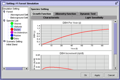
Figure 44: Growth Function Panel

3.3.5. Allometric Relations

DBH-Height is power function and DBH-Crown Width is linear function.

Height functions
The formula of height follows:

Height = alpha_h * DBH ^ beta _h

Crown Width functions
The formula of crown width follows:

Crown_width = alpha_cr + beta_cr*DBH

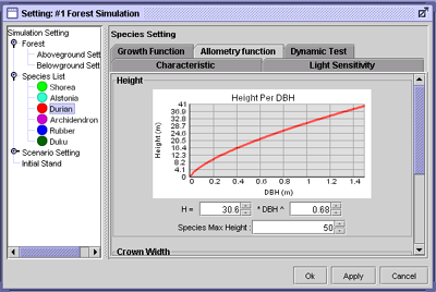
Figure 45:Profile Function Panel

3.3.6. Dynamic Test

Simple test of tree profile evolution over time and light condition can be tested here. Test Simulation in Dynamic Test.

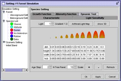
Figure 46: Dynamic Test Panel

The light option set the average of light received by this tree overtime, neglecting the spatial distribution of light. Here you can see the effect of light amount on dbh growth over time.

Artificial Light Map option gives a more advanced test. Here you can set the distribution of light over the crown by accessing a virtual hemispherical photograph describing the sky vault as viewed by the tree. Note that this is constant over time (whereas in the real condition it would be dynamically changing following the tree growth and environment dynamic evolution).

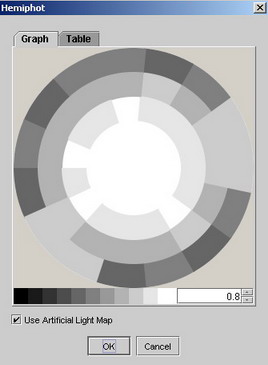
Figure 47: Artificial Light Map

Light Gradient is computed as the average ratio of light between vertical and the series of inclinations explored. Hence a light-gradient value of 1 would indicate NO light gradient (apart from the one possibly imposed by the illumination model not considered) while in case of dense planting with no overhead shade, light gradient would tend towards 0.

Note: check "Use Artificial Map" checkbox to activate the light map. You can check the 3D animation visualization of the tree growth by clicking the Show 3D button, enter the maximum age for the tree (see Figure 48: Age Dialog Box) the 3D animation shows the evolution of the tree profile over time.

Figure 48: Age Dialog Box

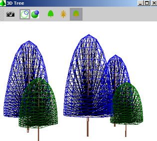
Figure 49: 3D Tree Visualization

3.4. Scenario Setting

Scenario definition may include general rules (“Simulation scenario”) or species specific rules (”species scenario”). Let’s explore each type.

3.4.1. Simulation Scenario

To change the simulation scenario select Scenario Setting node on the tree menu and the Scenario Setting panel will appear. The options in simulation scenario are:

• Allow Mortality
  Check the Allow Mortality box if you want to allow for mortality whiles the simulation running.
• Allow Recruitment
  Check the Allow Recruitment box if you want to allow for recruitment. Enter the starting time of recruitment.

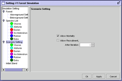
Figure 50: Plot Scenario Setting Panel

3.4.2. Species Scenario

In the species scenario species-specific management options can be set. Select a species for which you want to edit information by clicking the node under Species Setting node.

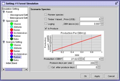
Figure 51: Species Scenario Panel

The options that can be chosen in the Species Setting panel are:

• Pioneer Species
  Check the Pioneer Species box if the species is a pioneer species, i.e. a species that will recruit saplings even if there are no sexually mature trees in the stand.
  Conversely, if a species is declared as non pioneer then it is allowed to regenerate only in the presence of adult trees of the same species.
• Timber Value
  Check the Timber valued box if the species has timber value. Input the price (in US$) in the given box.
• Logging
  Check the Logging box if the species can be logged. Input the DBH above (in m) value when the species is logged.
• Is Produce (fruit, latex, resin)
  Check the Is Produce box if the species can produce. The graphic Production per DBH (y) will show. Input the parameter for function
  production = (DBH * a) + b.
  Input value of production days per year. Check also “cut after produce days” box if the species will be felled (latex producing species) and enter the number of production days after which the tree will be felled.

3.5. Initial Stand

Once you have set-up a species list for your simulation, you need to plant trees. Go to the Initial Stand panel on the Simulation Setting window. Go to the Initial Stand panel on the Simulation Setting window. The Figure 52 below shows the Initial Stand window. There are three ways to plant the trees into plot:

3.5.1. Regular Plantation

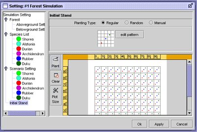
Figure 52 Initial Stand with Regular Plantation

To plant the trees regularly, use the pattern editor for design the plantation pattern. Click on “Edit Pattern” button to show the pattern editor. Figure 53 shows the plantation result with current designed pattern.

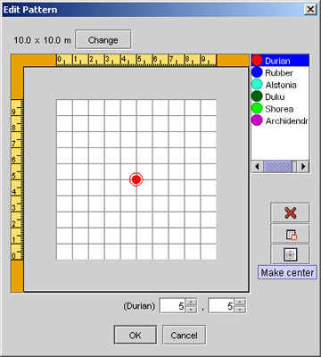
Figure 53 Plantation Pattern Editor

To edit the pattern, just select the species on the right top corner the click on the pattern plot. Click clear to remove the current pattern.

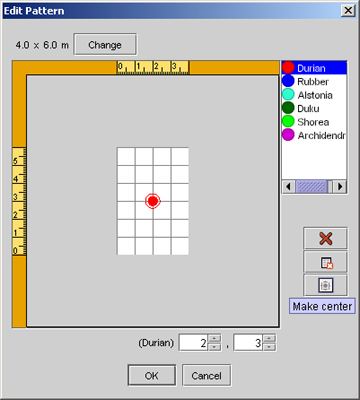
Figure 54 Regular Plantation 3x6m

If you want to create a regular pattern 3x6m plantation, change the pattern size by clicking the ”change” button. Put the tree on the center of the pattern plot (if you want make sure it was on the center of the plot, click on “Move to Center” button)

After you edit the pattern, click "Ok" then click "Plant" .

3.5.2. Random Plantation

If you choose plant randomly, the system will plant the species randomly. Check the Select column on the species you want to plant, type number of tree on Amount column, and click the Plant button. The system will plant the tree randomly.

You can plant more than one species. Figure 55 below shows that system will plant ten rubber trees, ten durian trees, and ten duku trees randomly.

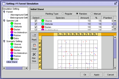
Figure 55: Random Plantation

3.5.3. Manual Plantation

If you choose to plant manually, you must click planting location in the planting area. Select species that you want to plant, and then click in the planting area on the location where the tree will be planted. You can plant any number of trees.

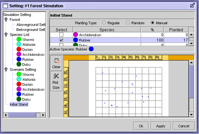
Figure 56: Manual Plantation.

You can delete a tree by selecting it, right clicking, and choosing “delete”. Or click on “Clear” button if you want to remove all the planted trees.

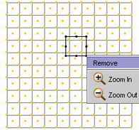
Figure 57: Remove Tree

3.6. Running the Simulation

3.6.1. Run Simulation

Simulation will be running for a specified number of steps (years). While the simulation is running, you can see the progress bar that indicates progress of simulation. To begin to run the simulation, you can click Start menu on Simulation menu or in the Control Simulation window.

Figure 58: Simulation Control Window

3.6.2. Stop simulation

There are several ways to stop simulation, such as

• Click stop button on Simulation Control window, or
• Select Stop menu on Simulation menu.

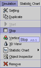
Figure 59: Stop Menu in Simulation Menu

3.6.3. Remove Simulation

This command closes the selected simulation on the Simulation List window, and if the simulation is unsaved, the program will ask whether you want to save the simulation or discard it.

There are two ways to remove simulation from the simulation list:

1. Select the simulation you want to remove. Right click, and option dialog will show, and then select Remove.
2. Select the simulation you want to remove from simulation list. Click Simulation menu, and then select Remove.
   
   
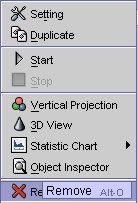
   Figure 61: Remove Menu in Simulation Menu

After you have done one of those steps, the Remove Confirmation dialog will show, and click Yes button to remove the selected simulation.

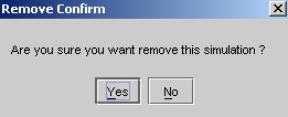
Figure 62: Remove Confirmation

3.6.4. Duplicate Simulation

For analysis reason, it is possible to duplicate a simulation, and run it after changing some management options. There are two ways to duplicate a simulation:

1. Select the simulation on the Simulation List window that you want to duplicate. Right click and an option dialog will show, and then select Duplicate menu.
2. Select the simulation you want to duplicate from the Simulation List. Click Simulation menu, and then select Duplicate menu.
   
   
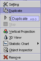
   Figure 64: Duplicate Menu in Simulation Menu

3.6.5. Save Simulation

You can save simulation information under two formats: simulation file (*.s) and simulation setting file (*.xml). Simulation file contains all simulation data including simulation setting and simulation result data, while simulation setting contains only the simulation setting.

To save the simulation, follow these steps:

1. Select the simulation
2. Click Save option on File menu
   
   
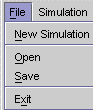
   Figure 65: Save Option on File Menu
   
3. The Save File dialog will appear, like in Figure 66.
   
   
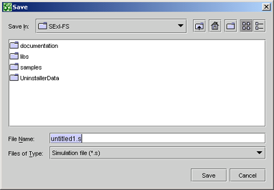
   Figure 66: Save File Dialog
   
4. Select the file type on Files of Types: simulation file (*.s) or simulation setting (*.xml).
5. Fill the file name on File Name.
6. Click Save button.

3.6.6. Open Simulation

To open simulation that has been saved before, click the File menu, and select open menu.

Figure 67: File Menu

The open dialog will show, like in Figure 68 below. Select the location and the file that you have saved before.

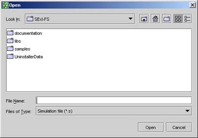
Figure 68: File Open Dialog