2 Model description and main algorithms

2.1 Main loop

The loop is run on a yearly time step. It starts with initialization phase, the initial trees are recorded into the module as individual objects. Next the trees crown attributes (Crown Form Index (CF) and Crown Position Index (CP)) are updated. Crown Form is an index of crown integrity and Crown Position is an index of light availability. Simulation data is then recorded after this step.

Tree growth is then computed (diameter, height and crown volume increment). At each step in time, for each tree a survival test is made. Finally at stand level a recruitment test is conducted.

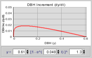
2.2 DBH Increment and growth reducers

DBH as a function of time (t) follows a Chapman Richards function:

And approximating DBH annual increment with the first derivative of DBH with respect to time (t) one can express dbh increment as a function of current dbh as follows:

One can note that maximum increment is then

which is attained when

 

Default initial diameter is one cm.

Potential DBH increment as defined above is reduced by the effect of aboveground and belowground competition. Thus the actual DBH increment is: dbh_inc_act = dbh_inc * growth_reducer

Growth reducers in this model are:

1. Light Stress (Crown Position Index)
2. Crown Form Index
3. Light gradient
4. Local fertility index
5. Tree Production Effect (competition for carbon allocation between growth and production of resin, latex, or fruit)
6. Belowground competition (based on local crowding)
7. Other possible growth reducers could relate to other ecological constraints such as pest pressure, diseases, etc… (not yet implemented)

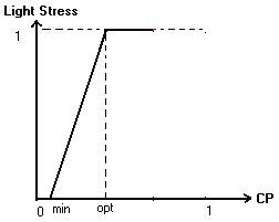
2.2.1 Light Stress

Light Stress factor value is derived from the curve below that is specific to each functional group:

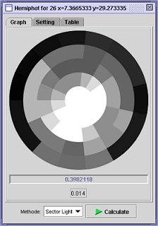
min = Minimum level for growth to occur
opt = Optimum level for growth

CP is Crown Position, which is an index of access to light. The computation of this light availability is explained in details in the SLIM section below.

In short Crown Position is computed based on a virtual hemispherical photograph that would be taken at tree crown base, the target tree crown itself being completely transparent.

Figure 2 Hemispherical
Photo

graph (left) compare with the model calculated (right) in high-resolution method.

Figure 3 Low resolution Hemiphot, shows a CP = 0.398 on range 0 – 1.

2.2.2 Crown Form (CF)

Crown Form is an index based on the ratio of actual crown size to normal crown size of a tree with same DBH. The crown size is defined by the surface area of the crown.

The difference between actual and normal crown size may result from encroachment from neighboring crowns, suboptimal light level or asymmetric development of the crown. The asymmetric development of the crown is explained in STRETCH model part below.

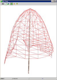
Figure 4 an asymmetric development of crown shown on the model

2.2.3 Belowground Crowding Index

Below ground competition is based on the following simple assumptions.

1. Root influential zone of a tree is proportional to its size and symmetric in shape (circular)
2. A crowding index is computed for any tree based on the overlap of neighbors' IZ with target tree influential zone
3. 3 More competitive species have relatively larger IZ (i.e. higher resource capture efficiency)
4. Overall below-ground crowding index effect on growth is site specific (dependent on overall level of resources)

The relationship used to relate growth reduction to below-ground crowding index is illustrated in the graph below, where s is the site index fertility value.

Relationship used in SExI-FS to compute growth reduction as a function of BGCI

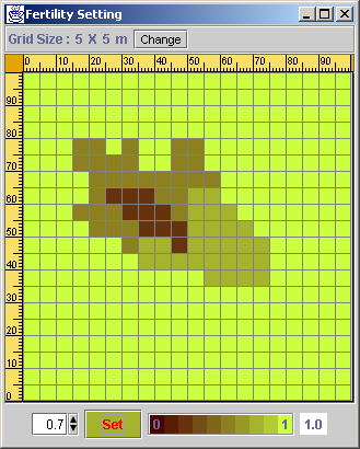
2.2.4 Fertility

Local variation of soil fertility can also be simulated. A soil fertility map can be entered manually for each cell of a grid covering the plot or read from a text file. Missing data are interpolated using bilinear 3 dimensional interpolation (Press, Teukolsky et al. 1992). Fertility values are between 0 to 1, a fertility of one meaning there is no local soil fertility related limitation (in addition to the overall fertility level defined in the step above). The fertility experienced by a tree will then depend on tree position in the plot. Fertility index used for computing reduction in growth of a particular tree is simply the average value over the cells included in the tree's influential zone. All cells which center is included in the crown projection are used in mean fertility calculation.

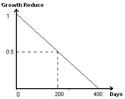
Figure 5 Fertility Map

2.2.5 Tree Production Effect

For now, Production Effect is implemented only for Rubber trees. Annual DBH increment decreases with increasing tapping frequency. Research on rubber trees shows that after 200 days of tapping, DBH increments decrease by about 50% (see review in (Grist, Menz et al. 1998) and data in Vincent et al. (2003) in prep). The figure below depicts the relation between the Growth Reducer value and the number of tapping days per year.

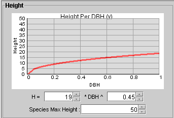
2.3 Height Increment

Height is a function of DBH:

Figure 6 Height -DBH function

Thus height increment, which is the function of DBH increment, is:

And the height increment corrected by the factor of light gradient is:

Where c is the light gradient adjustment factor: Where:

• flexi is a parameter which measures the ratio of height growth rates under the most contrasted light gradients (0 and1)
• light_gradient:
  
  where i is the inclination index (n inclinations including vertical direction) and j is the azimuth index (m being the total number of azimuths) in the sectoral light map. Hence a light_grad value of 1 would indicate NO light gradient (apart from the one possibly imposed by the illumination model not considered) while in case of dense overhead shading, light_gradient would tend towards 0
• sensi is a measure of how sensitive the species is to the vertical light gradient, sensi > 1 (e.g. 2) typical of a shade avoiding species and sensi < 1 (e.g. 0.5) of a shade tolerant species

and the break_function is defined as follow:

, where hc is current height, hMax is asymptotic height and k curvature parameter that is taken to be 20 for all species

Figure 7 Height Break Function

Enhanced height growth is achieved to the expense of dbh increment. Assuming that total stem biomass scales isometrically with the product of stem cross sectional area and tree height, the maximum possible height increment is then limited by actual dbh increment.

Maximum possible height increment is calculated as follows (i.e. height increment in case stem volume increment is entirely due to height increase [dbh_inc=0])

(ii) height_inc_max =

Note that max_height increment is independent of tree current slenderness!

Then actual height increment is:

height_inc_actual = Min(height_inc_gradient, height_inc_max)

Adjusting the actual dbh increment as the factor of slenderness:

if height_inc_actual = height_inc_max then dbh_inc_actual = 0

If height_inc_actual < height_inc_max then

dbh_inc=

Where s is the slenderness coefficient (current height/height of reference tree grown in the open) DBH, ?DBH, H, ?H refer to dbh, dbh_inc, height and height_inc of reference tree.

2.4 Crown Growth

A tree crown is represented as a deformable solid. Crown deformation can be global in response to increased vertical light gradient or local in response to radial anisotropy of incident light or spatial constraint.

Local deformation is mediated via a set of vectors stemming from crown base and subtending the crown envelope. Extension of the subtending vectors is affected by local light and space availability as determined by species-specific parameters.

Detailed explanation on how the crown is growth can be found in the STReTCH module section below.

2.5 Latex Production

So far only latex yield of rubber has been implemented. The relationship between size (DBH) and maximum latex yield is considered to be linear (Vincent, Wibawa et al. 2000):

Latex production is considered to decrease after a certain number of tapping incisions due to bark consumption and diseases, etc….

By default, the decrease in latex production is set to start after + 2000 days of tapping (say ten years of intensive tapping) and latex flow will completely dry up after + 8000 days of tapping. Then prediction of actual latex production after corrected by frequency of tapping (f):

and 0 if >8000 days

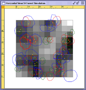
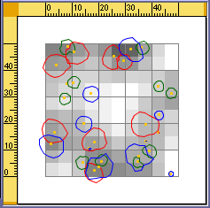
2.6 Recruitment

The plot is divided into a grid of cells (default size 5 by 5 m). For each cell at each time step a coarse index of light availability is computed based on overhead light of target cell and 8 immediate neighbors (a single vertical direction originating from center of cell is explored for each cell).

A further option (NOT RECOMMENDED) is to compute light availability at ground level using hemiphot light calculation model (see SLIM section) in point values are used instead of averages over 9 neighbouring cells.

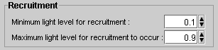
Figure: Light map for recruitment test shown in SExI GUI

The recruitment rate is determined at species level. The recruitment rate is the proportion of suitable "gaps” that are filled by a particular species at each time step. It does not depend on number of adult trees of the same species Suitability for recruitment is a functional group characteristic and is based on minimum and maximum light levels (calculated as defined above). Location of newly recruited seedling/sapling is randomly chosen within the range of suitable locations.

If the species is not a pioneer then it is allowed to regenerate only in the presence of adult trees of the same species. If it’s a pioneer than it can regenerate anytime.

Figure: GUI for recruitment parameters

2.7 Mortality

Survival probability is computed from two parameters: Min survival probability and m. Min survival probability is the survival probability value of a completely suppressed plant (no growth). m is aparameter affecting curvature of the relationship between growth rate and survival probability.

Min_sp is the survival probability value of a completely suppressed plants (showing no growth). This minimum probability increases with the ratio between actual and maximum growth rate r:

Where m is mortality modifier

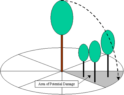
Fig : Relationship used in SExI to relate survival probability to growth rate relative to free growing tree of similar size.

In addition, systematic mortality is assumed once tree crown size has reached 5% of normal crown size.

The trees that don't survive enter the fall module.

The fall module deals with secondary damage due to tree fall. The direction of fall is random. Any tree smaller that 0.9 times the height of the falling tree and which is located in the area of potential damage is damaged. Area of potential damage is a sector defined by the direction of tree fall and the crown width of fallen tree and initial position of tree

All potentially damaged trees (see above) less than half the size of the falling tree are killed, whilst all the others are merely damaged. Tree damage here means a deterioration of crown form (up to ca 50% decrease of crown volume). This is achieved by dropping half side of the VBTs.