Tutorials

Beginner-Level Exercises for New Users


This part is an introduction to FALLOW user interface in MS-Excel. All exercises are aimed to familiarise you (technically) with the user interface of FALLOW model in MS-Excel using very simple cases without trying to interpret the parameters and the results intensely. The last exercise contains icons legend used in FALLOW interface for your reference. This introductory part contains 6 exercises, started from the easiest one.

1. Getting started with FALLOW

2. How to adjust your local attributes

3. How to select the working maps from available data in the list

4. How to modify input parameters

5. How to extract and retain the current results

6. Icons legend

1. Getting started with FALLOW


INTRODUCTION: When you’ve just installed FALLOW into your machine and have not made any changes on the parameters, you will get all parameters have been adjusted to run simulation of a simple scenario. In this simple scenario you will simulate if only shifting cultivation system practiced by a small number of people who occupied an initially forested landscape with the size of 10x10 grids. To introduce you with the user interface of FALLOW, we will start to run such simple scenario and see the results.

· Execute the FALLOW model by double-clicking its shortcut provided on your desktop:

· User interface of FALLOW model has been developed using macro programming in MS-Excel. Hence, please select Enable Macros when you have the macro notification message.

· Click the Run button available on the sheet “Main Menu” or any others.

· Confirm to run the batch file by pressing OK if you have a warning message.

· Simulation will be run for 100 steps in a DOS mode. Just wait until all running process done.

· Now, check the outputs of this simple run:

· From the sheet “Main Menu” or others, click the Output button .

· Click the button “Succession & Landuse/cover Change”.

· Click the blue square button at the left side of the row “Landcover change map” and confirm to run the batch file by pressing OK.

· You should see a totally forested landscape with 3 settlements (red, see legend on its left frame) displayed in PCRaster displaying window:

· To see the dynamics of the landscape over 100 years, click the Animate button . You should see the landscape starts changing.

· Close this PCRaster map-displaying window and back to your Excel.

· Still from the previous sheet, click the red square button at the left side of the row “Forest area (pioneer-primary)” and confirm to run the batch file by pressing OK.

· You should see the plotting graph of forests area based on their successional stages. The order of the legend from top to bottom is sorted based on these successional stages: pioneer forest (red line), young secondary forest (yellow line), old secondary forest (green line), and primary forest (cyan line):

· Close this PCRaster plotting window and back to your Excel.

· Still from the previous sheet, click the red circle 3D button at the left side of the row “Landcover change map” and confirm to run the batch file by pressing OK.

· You should see the landscape in a 3D view:

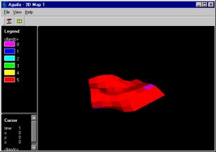
· In this 3D view, you can also see the dynamics of the landscape over 100 years by clicking the Animation button .

· Close this PCRaster map-displaying window and back to your Excel.

· In this exercise, you’ve just learnt on how to run and how to see the outputs. As your summary, 3 types of output representation have been provided:

1. The blue-square button is for outputs in form of 2D maps.

2. The red-square button is for outputs in form of graphs.

3. The 3D-red-circle button is for outputs in form of 3D maps.

· Now, explore other outputs by yourself.



2. How to adjust your local attributes


INTRODUCTION: FALLOW has been developed as generic as possible, hence we avoid to make any specific parameters in our model. This local setting feature was made to ease you to understand some parameters based on your local conditions.

· Click the Local Setting button available on the sheet “Main Menu” or any others.

· It will bring you to a sheet, on which you can adjust some local attributes according to your local condition. Attributes that can be adjusted locally are:

1. Currency

2. Crop types (FALLOW allows you to simulate 4 types of crop)

3. Plantation types and each of their products (FALLOW allows you to simulate 2 types of plantation)

4. Type of agroforestry and its main product

5. The main product from NTFP gathering activities

You can also make some remarks regarding simulation scenarios you want to run in the right table.

· To see the effect, try to change the currency unit from IDR into $

· Go to the sheet “Input Menu” by clicking the Input button
· Click the Market button.

· Notice that the price unit for the market parameters is now changed into $/kg.

· Try to modify other local attributes and explore by yourself which input/output parameters will be affected by the change.



3. How to select the working maps from available data in the list


INTRODUCTION: FALLOW is a spatially explicit model that requires spatial data formatted in raster data. In this part, you will exercise to use three different input maps, which have been provided. You will be trained on how to create and to prepare some input maps in more advanced tutorials.

· Click the Input button available on the sheet “Main Menu” or any others.

· Click the Spatial Data button.

· Right scroll the sheet to the table “input map”.

· From this table, three working maps are available: 10x10 grids of maps, 100x100 grids of maps, and real size of maps taken from Sumberjaya. Choose 100x100 grids of maps from the list by following these steps:

· Click the red circle button above the list 100x100:

· You will see that the above action will transfer the file name from the selected list into the list File name. Those files will be renamed according to the file names used in the model script (fallow$$.mod) using DOS command in a batch file (minput.bat). Hence, to modify the batch file, you must update your previous action by clicking the blue circle button available under the column list “File name” and always confirm to make a rewrite saving to the existing text file by selecting Yes, Save, Yes respectively.

· To activate the renaming batch file you have to execute Send maps button .

· Run the simulation by clicking the Run button . You should find that the running speed is getting slower. See some of the results following the previous exercise (Getting started with FALLOW).

· Try to repeat these steps for Sumberjaya maps but please, be ware that size of the maps will really affect the speed of simulation, so please reset the map to the simplest one (10x10) for the next exercises after your trial in this exercise.



4. How to modify input parameters


INTRODUCTION: In this exercise, you will learn on how to modify input parameters. Using simple scenario (shifting cultivation scenario), you will simulate if population density of people who live on the landscape increased.

· Before you start your modification, please repeat to run simple scenario using 10x10 grids of maps and let other parameters like what they are. For running the simulation, click the Run button . Please refer to the previous exercise (Getting started with FALLOW) if you get lost on how to run simulation.

· Check the output of this run by clicking the Output button from the sheet “Main Menu” or others.

· Select “Food Security” button.

· Click the red-square button at the left side of the row “Food sufficiency and its cumulative” and confirm to run the batch file by pressing OK.

· From the plotting graph, you should see the red line, which represents the current annual food sufficiency, and the yellow line, which represents the cumulative food sufficiency. From the cumulative food sufficiency, you should notice that with current population density, the carrying capacity of the landscape is stable enough for 100 years.

· Now, start to increase the population density:

· Close your graph-plotting window and back to your Excel.

· Click the Input button available on the sheet “Main Menu” or any others.

· Click the Population Dynamics button.

· Change the value of “Initial population density” from 15 into 45 and let others like what they are.

· Update your change by clicking the Updating button provided at the bottom part of the table, and always confirm to rewrite the existing text file by selecting Yes, Save, Yes respectively.

· Run the simulation by clicking the Run button .

· Repeat the above steps to see the output of “Food Security” and compare the current result with the previous one. What did you find with the carrying capacity of the landscape in providing food if human population increased?



5. How to extract and retain the current results


INTRODUCTION: In the previous exercises, you have learnt on how to see the simulation results in form of plotting graphs using features provided by PCRaster. In this exercise, you will learn on how to extract all current results into Excel spreadsheet, so that you will be able to plot some output parameters and make further analyses by yourself using MS-Excel’s features. You will also learn on how to save the current results of land-cover dynamics in form of maps in some defined directories.

· Click the Output button from the sheet “Main Menu” or others.

· Click the “Update current output in Excel” button and wait until the extraction process done. The process may take time. At the end of the process you have to confirm to make a rewrite saving to the existing text file by selecting Yes, Save, Yes respectively.

· Click the “Save current landcover maps in defined output directories” button and confirm to run the batch file by clicking OK.

· Click the “Go to current output button” to see all current outputs in tabular data.

· Click the “Go to all saved outputs” button to see all retained outputs in tabular data. Number in the table indicates the sequence number of simulation scenarios you have run and saved.

· Back to the sheet “Output Menu” by clicking the Output button .

· Click the “See retained landcover maps from some scenarios” button to see retained land-cover maps from some scenarios.

· Since you have just saved the maps from one run, you can only see the maps from the first row (scenario number 1). Just click the blue-square button if you want to see the 2D maps or the 3D-red-circle button for 3D maps. Name of the scenarios can be made by adjusting the local setting (see: How to adjust your local attributes).



6. Icons legend