The following information is based on Minasny et al. (2003).

We demonstrate this approach by showing an example of projecting the influence of climate change on soil C level in a region of New South Wales (NSW), Australia. The baseline SOC concentration map (0–50cm) was derived using legacy soil data collected in a nationwide database. A map was derived using a rule-based model based on the legacy data and environmental covariates with a grid spacing of 250m (Wheeler et al., in press). Climate information was found to be important predictors in the spatial prediction model. See Wheeler et al. (in press) for the techniques involved in the mapping. We focused on an area of 49,000 ha in the southern part of NSW (Fig. 1) and estimated the likely change in soil carbon with climate change. We used the 50th percentile of the estimated likely change in the mean annual temperature (MAT) and MAP by 2030 (relative to 1990 levels) for the corresponding area of NSW (Watterson et al., 2007). For a high emissions scenario, the MAT is expected to increase 0.6–1 °C (average 0.8 °C) and MAP to decrease 2–5% (average −3.5%). Using this information, we adjusted the climate covariates and recalculated the SOC concentration from the rule-based model. The assumption in this case is that the C level is at a steady-state condition (amount of input is constant). The projected map shows that there is an average potential loss of 5 t of C per hectare. Such information will help decision makers to decide on alternative land-management techniques that could reduce this loss.

This empirical approach is a relatively quick and pragmatic way to pro- duce a first-cut scenario to predict the change in soil C. It has limitations compared with a dynamic simulation model, such as lack of feedback and possible extrapolation problems. Nevertheless, the scorpan approach has been locally calibrated, and any changes in the factors should reflect the changes in the predicted C.

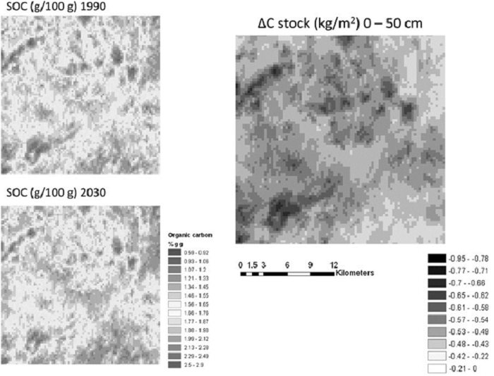
Figure 1. Map of the SOC at 0–50 cm in the southern part of NSW. The 1990 map was generated using a rule-based model based on legacy soil data and environmental covariates. The C level in 2030 was estimated under a likely climate change scenario (increase in the MAT and decrease in the MAP). The rule-based model was recalculated to reflect the climate change, and a map of likely C status in 2030 was produced. The change in carbon stock was then calculated based on estimates of the bulk density.

__________

Minasny, B., McBratney, A. B., Malone, B. P. 2013. Digital mapping of soil carbon, in Wheeler, I., et al. (eds.) Adv. Agron 118: 1-47.

Watterson, I. G., Weaver, A. J. and Zhao, Z. C. 2007. Global climate projections in S. Solomon, D. Qin, M. Manning, Z. Chen, M. Marquis, K. B. Averyt, M. Tignor and H. L. Miller (eds.) Climate Change 2007: The Physical Science Basis. Contribution of Working Group I to the Fourth Assessment Report of the Intergovernmental Panel on Climate Change. Cambridge University Press, Cambridge, United Kingdom, and New York, United States, pp. 747–846.