section 2 : basic principles

Simulation of tree shadows in agroforestry systems

F. Quesada, E. Somarriba, E. Vargas

CATIE
 Av. 7, c.15y 17, Casa 1561, San Jose, Costa Rica

Abstract

The understanding of how tree canopies intercept light is of prime interest for several disciplines. For instance, regeneration success of valuable tree species in a forest opening depends to a great extent on the illumination patterns at the forest floor. In agroforestry, it could help in the design of the planting arrays that most favourably influence the associated crop, and in the selection of appropriate experimental and sampling designs that take into account the fact that the associated crop is influenced by a neighbourhood of trees that may extend far beyond the nearest three or four neighbours.

Several attempts have been made to model light interception and shade projection by tree canopies. These studies have dealt with: I) determining the ground area under shade in relation to stand density, and 2) the orientation and length of shadows cast by trees at different latitudes, days and hours, etc. These studies provide some insights into appropriate planting patterns of trees and associated crops; but to be useful in selecting appropriate experimental and sampling designs, they should accurately keep track of shade movement on a coordinate grid system conveniently placed on the study plot. The model herein presented tackles this problem.

We developed a model which allows the calculation of the number of hours of both absolute shade, and overlaps cast at each coordinate point in the study plot over a number of days specified by the user. The plot can be a horizontal or tilted plane with a maximum size of 1 ha, and located at any latitude. The plot can be a lattice with a minimum size of 0.5X0.5 m. Any number of trees can be 'planted' on this plot following any spatial arrangement, but crown shapes have to be one of the following types: spherical, hemispherical, ellipsoidal, hemi-ellipsoidal, and conical. Solar movement can be simulated at any daily and hourly interval depending on the accuracy needed and on computer time available. A computer programme was written in BASIC to be run in microcomputers with a minimum RAM memory configuration of 256Kb. In this presentation an overview of model development is presented. Emphasis is placed on describing the geometric strategies adopt and in the presentation of the critical angles studied. An application of the model is presented.

Introduction

Tree shadows on an arbitrary plane are a function of tree parameters (tree height, tree coordinates, etc.), the position of the sun at any latitude and day of the year, and the orientation and slope of the plane. We describe an algorithm and computer programme that calculates the total hours of shadow in each small square of a plot over a given period of time which can be selected by the user. An optional subroutine provides the totals of shadow overlaps in each square over the period of time selected.

Shadow equations for a horizontal plane

We consider only trees with crowns of the following types: spherical, hemispherical, ellipsoidal, hemi-ellipsoidal and conical. The equations of the crown shadows are obtained with respect to a universal reference frame (an ordinary cartesian system of coordinates). The introduction of some intermediary cartesian systems is necessary before the equations are referred to the universal frame previously mentioned. These systems have their origins either at the center of the shadow (when the shadow is a symmetric figure and has a center) or at the base of the tree trunk.

The data that determine the tree shadow are: tree coordinates (with respect to the universal reference frame), trunk height (distance from the ground to the beginning of crown), crown height and crown diameter. Required positional data are latitude, day of the year and hour of the day. We assume that tree crowns are opaque; sun rays are parallel; that no corrections due to refraction of sun light in the atmosphere are necessary; and that there is no difuse radiation; that trunk width can be neglected so the only shadow that the tree produces is due to the crown.

Shadow equations for a tilted plane

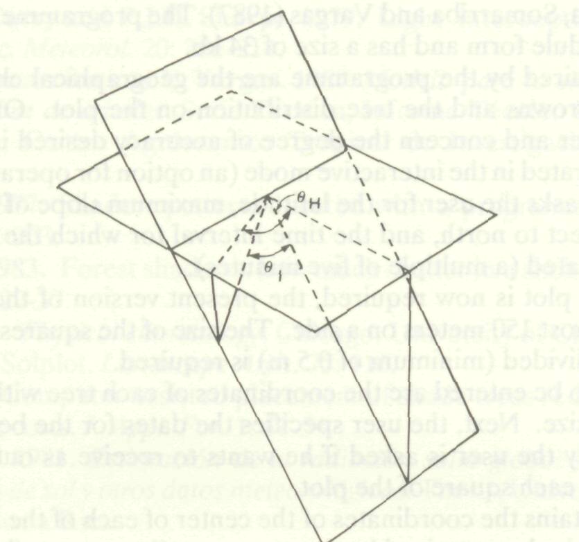
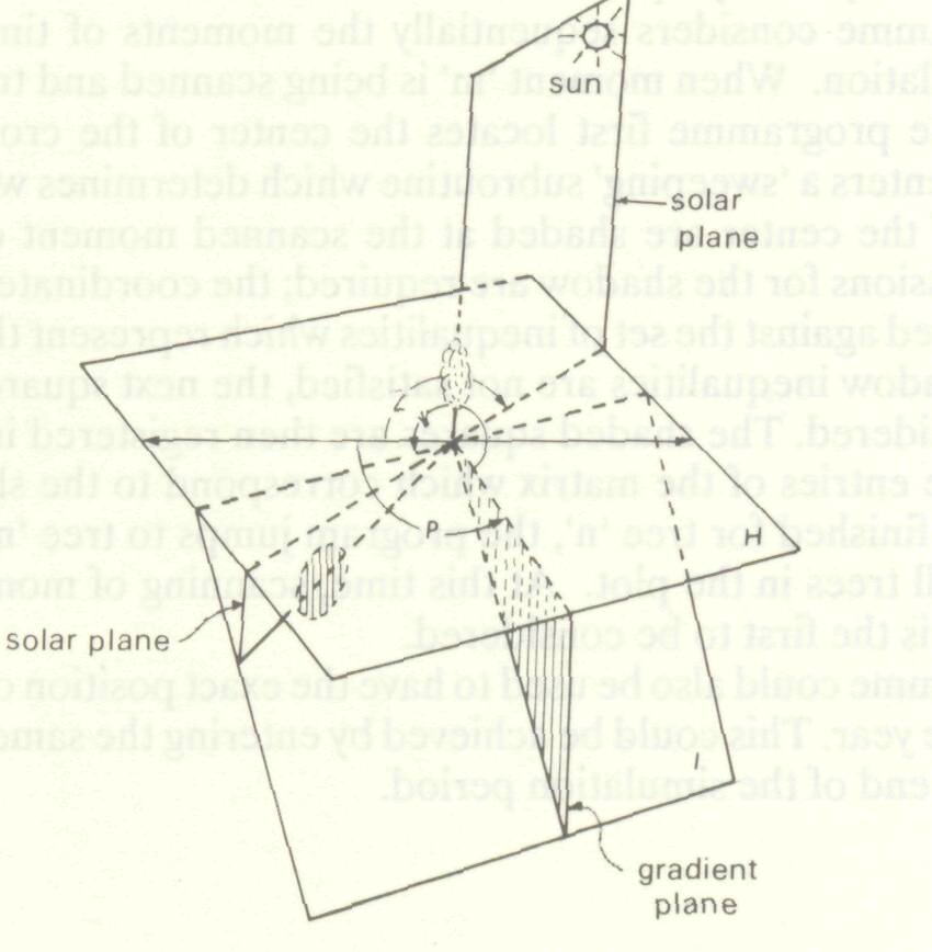
A general strategy for describing shadows on tilted planes has been developed, based on the concepts of a virtual shadow and a generalized change of coordinates. A virtual shadow is the one that the crown would project on any imaginary plane. When we deal with a tilted plane we can consider the virtual shadow over an imaginary horizontal plane. If this virtual shadow is thought of as a real opaque plane object capable of obstructing light rays, then it should also be capable of projecting a shadow coinciding with the real shadow of the crown.

If one considers now two reference frames, one in the real tilted plane and the other in the virtual horizontal plane, a generalized change of coordinates can be defined as a function which assigns to every point in the virtual plane its shadow in the tilted plane. This change of coordinates can be applied to the equations of shadows in the horizontal plane to render the corresponding equations in the tilted plane. One advantage of this method is that it is no longer necessary to compute the equations for the tilted plane case by case. One further advantage is that as soon as one has need for computing new equations for shadow types not included hitherto, it is sufficient to compute them for the horizontal case only.

The generalized coordinate transformation developed depends on the slope of the plot; and on its orientation with respect to north, defined as the angle between the north axis and the horizontal projection of the line of maximum slope in the plot. The generalized change of coordinates has been performed by means of simple trigonometric calculations. In order to make these calculations clear we have simultaneously considered four basic planes attached to each tree: the real tilted plane where the tree is located; a virtual horizontal plane which passes through the basis of the trunk; a vertical plane containing the trunk and which is parallel to the lines of maximum slope of the tilted plane (this plane is called 'gradient' plane); and finally a vertical plane which contains the trunk and which is parallel to the sun rays (referred to as 'solar' plane) (Figure 1).

The transformation shows that when crowns are projected in a tilted plane they undergo an amplification-contraction effect as well as a 'twisting' effect: the line containing the shadow of the trunk is no longer a symmetry axis for the shadow (Figure 2). This 'twisting' effect is not equivalent to a rotation of the shadow. The general transformation is linear and so it can be expressed in matrix form.

Figure 1 Geometry of tree shadow on a tilted plane.

Details of the mathematical development are presented in Quesada, Somarriba and Vargas (1987).

Figure 2 Relationship between virtual shadow and the real shadow on a tilted plane.

Development of computer programme

We now describe a programme that can be run on a personal computer of about 256K RAM memory. A detailed discussion of the algorithm as well as a list of the programme is given in Quesada, Somarriba and Vargas (1987). The programme is written in Microsoft BASIC in module form and has a size of 34 kb.

Input data required by the programme are the geographical characteristics of the plot, the type of crowns and the tree distribution on the plot. Other input data are selected by the user and concern the degree of accuracy desired in the output. If the programme is operated in the interactive mode (an option for operating it in batch form is offered), then it asks the user for the latitude, maximum slope of terrain, orientation of slope with respect to north, and the time interval for which the position of the sun should be recalculated (a multiple of five minutes).

The size of the plot is now required, the present version of the program allows a square plot of at most 150 meters on a side. The size of the squares into which the plot is going to be subdivided (minimum of 0.5 m) is required.

The next data to be entered are the coordinates of each tree with the description of crown shape and size. Next, the user specifies the dates for the beginning and end of the period. Finally the user is asked if he wants to receive as output the amount of shadow overlap in each square of the plot.

The output contains the coordinates of the center of each of the squares of the plot; the total hours of shadow received by the corresponding square (in hours) during the period of simulation (e.g., 30 of March to 20 of November); and the total hours of shadow overlap during the simulation period.

A brief description of the algorithm

The plot is represented in the computer memory as a matrix. If shadow overlaps are required, an extra matrix of the same size is needed. The program proceeds 'tree by tree', instead of 'square by square'.

The programme considers sequentially the moments of time which conform the period of simulation. When moment 'm' is being scanned and tree number 'n' is being considered, the programme first locates the center of the crown shadow. The programme then enters a 'sweeping' subroutine which determines which of the neighbouring squares of the center are shaded at the scanned moment of time. At this point, analytic expressions for the shadow are required; the coordinates of the center of each square are tested against the set of inequalities which represent the shadow at this given moment. If shadow inequalities are not satisfied, the next square in the sweeping subroutine is considered. The shaded squares are then registered in the matrix, a 1 being added to those entries of the matrix which correspond to the shaded squares. When this process is finished for tree 'n', the program jumps to tree 'n +1' and so on until it finishes with all trees in the plot. At this time, scanning of moment 'm +1' starts and tree number 1 is the first to be considered.

The programme could also be used to have the exact position of shadows at any given time during the year. This could be achieved by entering the same date and hour for the beginning and end of the simulation period.

References

Knapp, R.H. and R.L. Williamson. 1984. Crown shadow area equations. For. Sci. 30:

284-290. Mann, J.E., G.L. Curry and P J.H. Sharpe. 1979. Light interception by isolated plants. Agric. Meteorol. 20: 205-214.

Quesada, F., E. Somarriba and E. Vargas. 1987. Modelo para la simulacion de patrones de sombra de arboles. Serie Tecnica, Informe Tecnico No. 118. Turrialba, Costa Rica: Centro Agronomico Tropical de Investigacion y Ensenanza (CATIE).

Satterlund, D.R. 1977. Shadow patterns located with a programmable calculator. J For. 75: 262-263.

Satterlund, D.R. 1983. Forest shadows: how much shelter in a shelterwood? For. Ecol. Manage. 5: 27-37.

Sellers, W.T. 1965. Physical climatology. Chicago: University of Chicago Press.

Wagar, J.L. 1985. Solplot. Landscape Arch. 75:116.

Wagar, J.L. 1986. Computer-assisted placement of shade trees reduces home heating and cooling costs. J. Appl. For. 1: 51-54.

Wright Gilmore, J. 1981. Estimacion de la radiacion solar global en Costa Rica utilizando horas de soly otros datos meteorologicos. Thesis, University of Costa Rica, San Jose, Costa Rica.