![]()
An e-publication by the World Agroforestry Centre
METEOROLOGY AND AGROFORESTRY

|
|
An e-publication by the World Agroforestry Centre |
|
METEOROLOGY AND AGROFORESTRY |
|
|
section 3 : regional examples Environmental driving variables of ecosystems and their distribution on a complex terrain A. Hocevar and L. Kajfez-Bogataj
Department of Agronomy, Edward Kardelja University Abstract Using an example of general model of ecosystem productivity, the role of environmental driving variables is stressed. Use of the particular model when only light is the limiting factor is presented for a few places in Slovenia, Yugoslavia. The importance of other limiting factors, e.g., water, is illustrated; and simple methods of how to incorporate it in the model are presented. Several examples are given of how to assess the peculiarities of the environmental driving variables in a complex terrain which must be known for assessment of ecosystem productivity of an area.
Since the first agricultural fields were established in ancient times, their productivity has been monitored in one way or another. Farmers and foresters and their ancestors tried to increase the productivity of ecosystems they manage. At first the understanding of ecosystem functioning has been vague and more or less at the descriptive level. Later on statistical relations among biological variables and environmental ones have been determined and models on these bases developed (Robertson 1983). In the last two decades, the understanding of ecosystem functioning has been one of the main goals of research in this field. A further development is dynamic modelling of the ecosystem and its simulation on computers (de Vries 1982). These models are based on biological, physical and chemical principles. They try to explain the ecosystem functioning by selection of main variables and by the study of their interrelations. They have been applied in various versions at many locations throughout the world (Robertson 1983). In the present contribution we extend the concept of ecosystem modelling from a particular location to an area with mesoscale dimension. To illustrate this we present a general model of ecosystem productivity and a particular model when light is the limiting factor. The model is applied to locations in north-western part of Yugoslavia. The importance of another limiting factor water is stressed and simple methods of incorporate it in the model are presented and the obtained results discussed.
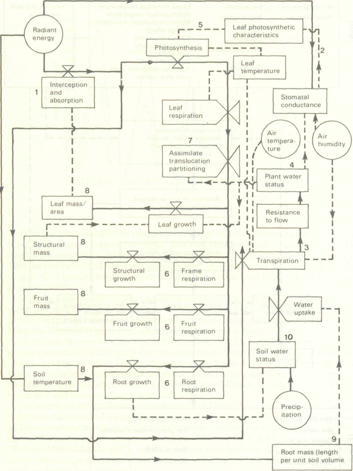
The productivity of a plant canopy ecosystem (P) is a function of biotic parameters describing phytometrical, physiological and optical characteristics of a plant canopy; and abiotic parameters describing the soil and meteorological environment. The influence of management is implicitly included in the biotic and abiotic parameters. Since all parameters are interrelated, for producivity (P), we can write: P = f(Bl,Sm,Mn) (1) where l, m and n are the numbers of biological, soil and meteorological parameters, respectively. According to Gaastra (1963), the productivity sought as net photosynthesis is a function of weather. It can be separated into photochemical processes driven by photo-synthetically-active radiation, biochemical processes governed by temperature of the plants and transport phenomena among the plants and their environment as determined by morphological and physiological characteristics of plant canopy, and the wind and temperature regime in and above the canopy. Some interrelations of this function are already known but a complete knowledge of these complex relations is still far ahead. Models based on realistic simplifications of the ecosystem have been derived and many of them are at work in the world (Robertson 1983). Among simplified dynamic models we can distinguish four types: when light is the limiting factor (level 1); when water is the limiting factor (level 2); when nitrogen is the limiting factor (level 3); and when phosphorus is the limiting factor (level 4) (de Vries 1982). A schematic presentation of a general model of plant production in relation to weather (production level 1) is given according to Landsberg (1981) on Figure 1.
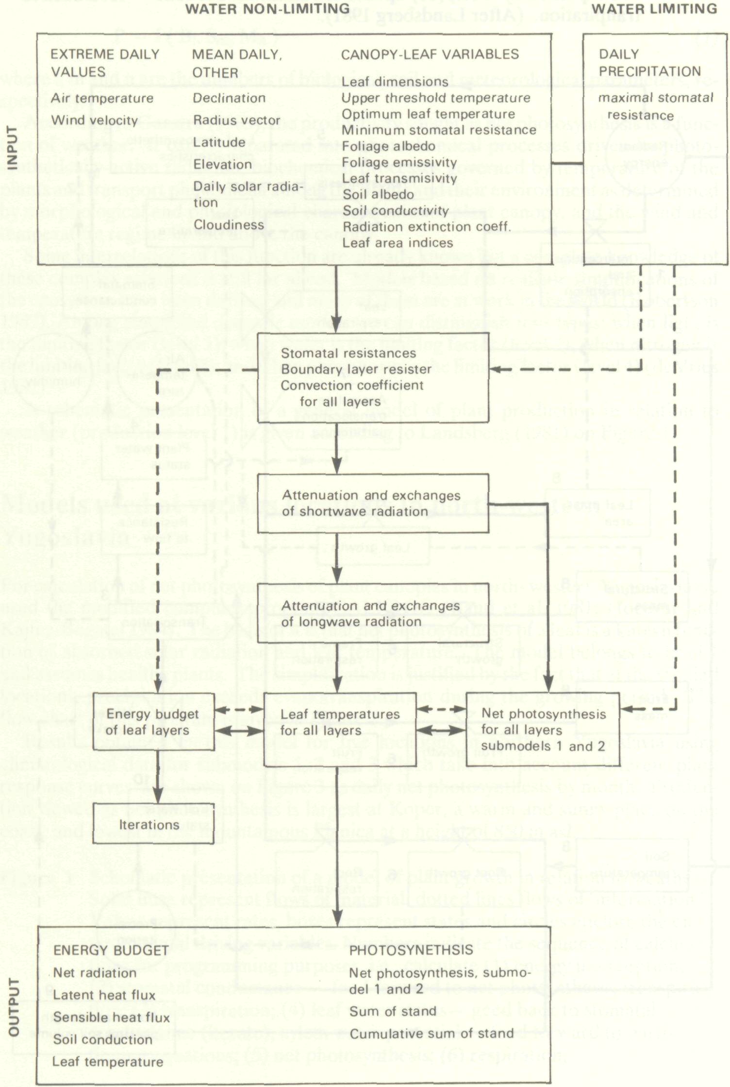
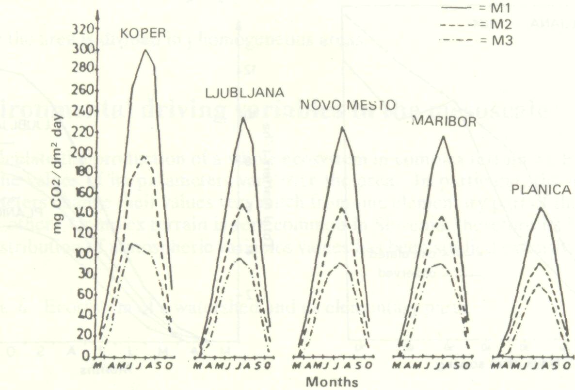
For calculation of net photosynthesis of plant canopies in north- western Yugoslavia we used the modified computer program CALPROD (Band et al. 1981; Hocevar and Kajfez-Bogataj 1984). The basis of it is that net photosynthesis of a leaf is a known function of absorbed solar radiation and leaf temperature. The model belongs to level 1 and assumes healthy plants. The simplification is justified by the fact that at the studied locations, precipitation exceeds evapotranspiration during the growing period. The flow chart of this program is given in Figure 2. Results obtained by this model for five locations in northern Yugoslavia using climatological data for submodels 1, 2 and 3 which take into account different plant response curves are shown on Figure 3 as daily net photosynthesis by month. Production viewed as net photosynthesis is largest at Koper, a warm and sunny place on the coast; and lowest in the mountainous Planica at a height of 850 m asl.
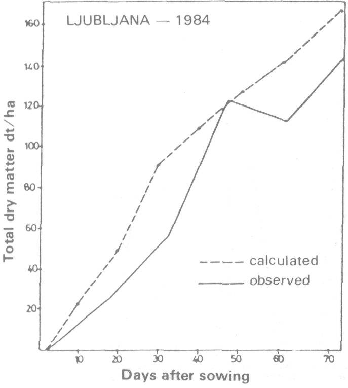
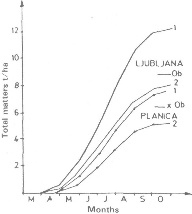
With the same model we also calculated net photosynthesis of a beech forest at two elevations using biological variables for locations at Ljubljana and Planica. Comparison of observed and predicted net photosnynthesis shows fairly good agreement in spite of being the first trial (Figure 5) (Kajfez-Bogataj and Robic 1985). In general, the north-western part of Yugoslavia with large amounts of precipitation (yearly amounts 1250-1750 mm) does not experience drought although some years may show a shortage of water. During these dry years, there are negative effects on plant canopy productivity, viz., stomatal resistance will be larger, transpiration will be smaller and therefore temperature of leaves will be higher, diffusion of CO2 into stomata will be smaller and so net photosynthesis will decrease. We incorporated the shortage of water in CALPROD by using a minimum stomatal resistance calculated as a function of water balance. Thus, additional input data and additional computations are needed for the maximum stomatal resistance and the main terms of water balance equation, daily precipitation and daily evapotranspiration (Bringfeld 1980; Maticic 1977). Additional input data and their influence on particular computation steps of the computer program are schematically presented on the flow chart by dashed lines (Figure 2).
From data on daily precipitation and daily evapotranspiration we calculated minimum stomatal resistance as a linear function of time, the factor of proportionality being on the order of 2-7 s cm-1 day-1 beginning on the day when all the precipitation was used for evapotranspiration. Until this day, stomatal resistance had the minimum value given by the input data. An efficiency parameter was calculated from the minimum and the maximum stomatal resistance and the calculated minimum stomatal resistance for particular day. Since its value has to be between one and zero, we applied the cosine-squared function. Preliminary results obtained by the modified program which includes light and water as limiting factors show rather small changes in comparison with the previous ones except in Koper which is located on the Mediterranean coast. We speculate that the differences in water regime are not large enough from year to year and the model not sensitive enough to show a well-expressed influence of water shortage on net photosynthesis. In regions with large water shortages, we can expect that the mentioned modifications of the model will be of greater significance.
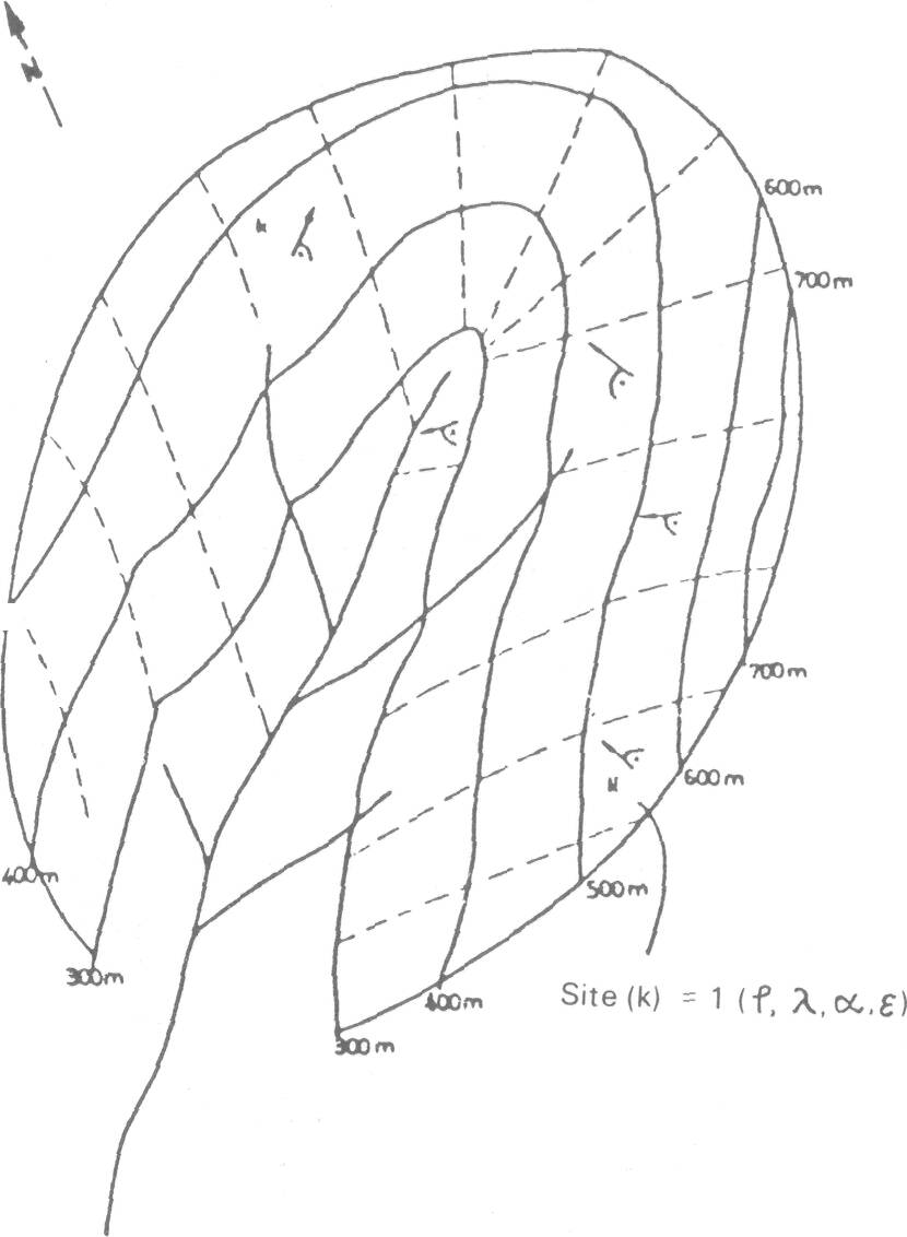
The model can be applied to a large area if all of its parameters do not change very much over the area or to a smaller area in complex terrain. In nature, an ecosystem of an area normally consists of (j) elementary parts (Figure 6) which are defined by different values of parameters and therefore different productivities (Pk) Pk = f(Bik,Smk,Mnk) (2) To obtain the productivity of an area we have to sum up the productivities of elementary parts:
where the area is divided in j homogeneous areas.
To calculate the production of a whole ecosystem in complex terrain we have to know how the values of its parameters vary over the area. In particular, the atmospheric parameters change their values very much from one elementary part of the ecosystem to the other. Complex terrain is very common in Slovenia; therefore its influence on the distribution of atmospheric variables values has been studied extensively. Some of these studies will be discussed giving methods for evaluation of atmospheric variables as a function of terrain or site.
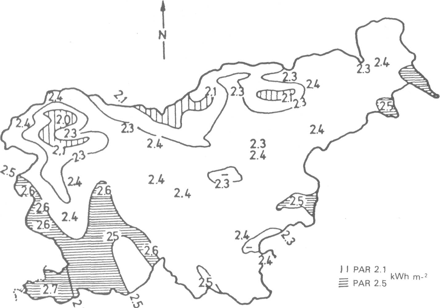
One such atmospheric variable is minimum temperature. It shows very distinctive features in valleys and basins on mornings after clear and calm radiation nights. A temperature inversion develop with air minimum temperature increase from the bottom of cold air lake basin. The rate is between 4.4 °C/100 m and 6.2 °C/100 m height along the slopes. These values resulted from measurements in Slovenia (Petkovsek et al. 1969) and in Pennsylvania, U.S.A. (Hocevar and Martsolf 1972) and are theoretically explained by Hocevar (1973). Photosyntheticallyactive radiation (PAR) determines photochemical processes (Gaastra 1963). We developed a method for estimating PAR for any site in complex terrain (Hocevar and Rakovec 1981). The method has the following steps: First, a map showing the areal distribution of PARh on a horizontal surface in the chosen period is prepared based on calculations from hourly measurements os sunshine duration at climatic stations (31 in Slovenia) and spatial features of convective cloudiness, fog and air pollution in the same time intervals. This is done for a typical day of every decade and every month of the year (Figure 7). Second, PAR of an element of sloping surface (PARs) is calculated as the product of ks and PARh, where ks is a function of azimuth and inclination of the surface. Both ks and PARh are functions of the treated time period, as well. PARS = ks (PARh ) (4) A matrix of coefficients ks was obtained from known values of PARs and PARh at lo-cations observing meteorological parameters (Hocevar and Rakovec 1979).
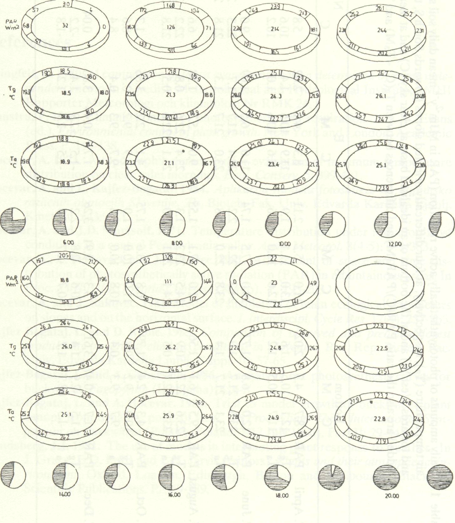
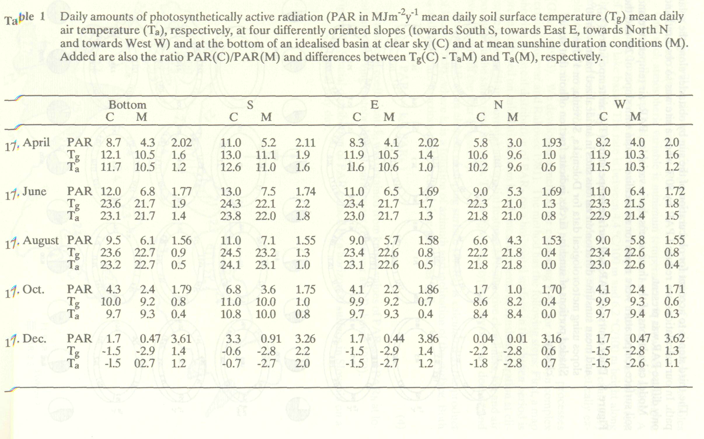
Model calculations of the three atmospheric variables, PAR, air temperature and soil surface temperature were made for an idealized basin with slopes of 20° and the observed mean duration of sunshine at Dolenjska, Slovenia. The results are given as daily courses ( Figure 8 ). Daily mean values are compared with clear sky values in Table 1.
Conclusions The results of modelling indicate that it can be a powerful tool for estimating ecosystem productivity. Dynamic modelling can be extrapolated from a point to an area. If the ecosystem is represented by its elementary parts, parameters defining those elementary parts must be known. This is especially true for highly changeable atmospheric variables in complex terrain. Some of the methods for evaluation of time and space distribution of those vital ecosystem parameters for which we give some practical examples have proved useful.
Bringfelt, B. 1980. A comparison of forest evapotranspiration determined by some independent methods. Swedish Meteorological and Hydrological Institute, SMHI Rapporter Meteorologi och klimatologi Nr RMK 24. Gaastra, P. 1963. Climatic control of photosynthesis and respiration. In L.T. Evans (ed.), Environmental control of plant growth. New York and London: Academic Press. P. 113-138. Hocevar, A. 1973. A topographic parameter for evaluation of minimum temperature distribution on clear calm mornings. Ecol. Conserv. 5: 399-401. Hocevar, A. and L. Kajfez-Bogataj. 1984. Aplikacija modela fotosinteze na klimatsko razlicnih obmocjih Slovenije. Zb. Bioteh. Fak. Univ. Edvarda Kardelja Ljublj. Kmetijstvo 43:9-23. Hocevar, A. and J.D. Martsolf. 1971. Temperature distribution under radiation frost conditions in a central Pennsylvania valley. Agric. Meteorol. 8(4-5): 371-383. Hocevar, A., Z. Petkovsek and J. Rakovec. 1981. Assessment of space and time distribution of photosynthetically active radiation (PAR) in mountainous areas. In Proc.XVII lUFRO World Congress (Kyoto). P. 193-203. Hocevar, A. and J. Rakovec. 1981. Model of simulation of main ecological parameters on slopes and on the horizontal surface J. Interdiscipl. Cycle Res. 12(4): 257-265. Kajfez-Bogataj, L. and D. Robic. 1985. Comparison of observed and predicted forest productivity in various climatic conditions in Slovenia. Res. Rep. Bioteh. Fac. Univ. Edvarda Kardelja Ljublj., Suppl. 10: 57-65. Kajfez-Bogataj, L. and A. Gaberscik. 1986. Analysis of net photosynthesis curves for buckwheat. Fagopyrum (Ljubljana). 6: 6-8. Kajfez-Bogataj, L. and A. Hocevar. 1986. Trial to model growth of buckwheat plant canopy from dynamic point of view. In Proceedings Third International Symposium on Buckwheat (Pulawy, Poland, 7-12 July 1986). Part II: 29-44. Landsberg, J J. 1981. The use of models in interpreting plant response to weather. In J. Grace, E.D. Ford and P.G. Jarvis (editors), Plants and their atmospheric environment. Oxford, London, Edinburgh, Boston and Melbourne: Blackwell Scientific Publications. P. 369-389. Maticic, B. 1977. Evapotranspiration studies on different crops and irrigation water requirements. Biotechnical faculty, University of Ljubljana, Final Technical Report P.L. 480 Grant No. FG-YU 212, Project No.E 30-SW-15. 221 pp. Penning de Vries, F.W.T. and H.H. van Laar (editors) 1982.Simulation of plant growth and crop production. Wageningen: Centre for Agricultural Publication and Documentation. Petkovsek, Z., I. Gams and A. Hocevar. 1969. Meteoroloske razmere v profilu doline Drage. Zb. bioteh. fak. Univ. Ljublj.16:15-24. Robertson, G.W. (editor). 1983. Guidelines on crop-weather models. World Climate Programme. World Meteorological Organization. 115 pp. |